Agricultural Statistics

PDF version of Notes

Available Versions of SAS

• PC Standalone Version – PC-SAS
  • Available for Windows ONLY – if you’re using a Mac, you will need to have a VM to emulate Windows to run this version
  • Available through CCS Software Distribution Centre – $135.00 for a new license and $75/year renewal license. This information was downloaded on June 3, 2019, please check https://guelph.onthehub.com/WebStore/Welcome.aspx for updated pricing and access information or email 58888help@uoguelph.ca for more information
• Animal Biosciences department ONLY
  • Access the server version of PC-SAS
• SAS University Edition
  • This is free for all academics to use. You can download the free version from https://www.sas.com/en_ca/software/university-edition.html
  • This is available for both Mac and Windows users
  • Please note, that you will be required to update this version every year.  SAS will send you a reminder notice, approximately 1 year from your installation date.
• SAS OnDemand
  • This is also free for academics
  • This is SAS’ in the cloud version of the University Edition
  • Environment is the same as the University Edition, the difference is that you are using the SAS service in the Cloud, all your files are stored in the Cloud and not on your local system, and you are using their computer resources NOT your own system – accessed through a web browser with your own personal login

What Parts of SAS do you have access to?

SAS is an extremely large and complex software program with many different components.  We primarily use Base SAS, SAS/STAT, SAS/ACCESS, and maybe bits and pieces of other components such as SAS/IML.

SAS University Edition and SAS OnDemand both use SAS Studio.  SAS Studio is an interface to the SAS program and contains the following components:

• BaseSAS – base SAS programming, DATA Step
• SAS/STAT – the PROCs used for statistical analyses
• SAS/IML – SAS’ matrix programming language
• SAS/ACCESS – allows you to interact with different data formats
• Some parts of SAS/ETS – time series analysis

If you are using the PC or Server SAS versions, you may have access to more than the modules listed above.  To see exactly what you have access to, you can run the following code:

Proc Setinit;
Run;

You will see the components available to you listed in the log window.

Also note the additional information available to you:

• License information
• Expiration date – very handy to be aware of, especially if you are running your own copy of your PC
• SAS components available to you

What does SAS look like?

There are a number of components to the SAS interface:

• Results and Explorer windows to the left
• Editor, Log, Output, and Results Viewer windows to the right, taking up most of the screen

What do each of these windows do?

• Results Window –  a Table of Contents for all of your results.
• Explorer Window – similar to Windows Explorer – allows you to navigate SAS libraries and files
• Editor Window – this is where you will spend most of your time, writing and editing program files
• Log Window – this window is extremely helpful, think of it as your best friend in SAS, it tells you what SAS has done every step of your program and processing
• Output Window – SAS versions 9.2 and earlier, use this window to display all results and output.  SAS 9.3 and higher use a new window called the Results Viewer.  All the results are presented in an HTML format.

How does SAS work?

SAS is divided into 2 areas:

• DATA step
• PROCs (short for PROCedures)

DATA step is all about data manipulation – one of the key strengths to SAS
PROCs – this is where you will find most of your statistical procedures.

How do you get data into SAS?

The primary reason we use SAS is to perform statistical analyses on some data.  However, we need to ensure that the data we have collected is brought into SAS correctly.  I’m sure you’ve heard of “garbage in, garbage out”?  This cannot be more truer than when you collect data and bring it into a statistical package.

There are different ways to bring data into SAS.  I will try to review and provide my thoughts on 3 different ways I see my students performing this task.  However, before we import data into any software package, we need to ensure the data is “clean” and in a format that will be accepted into the package.  So let’s talk about the most common way researchers enter their data – EXCEL.

Using Excel to enter data and Statistical Software packages

Most people use Excel to enter their data and that’s great!  The look of it is neat, ordered and we can do quick summaries, such as means and sums.  We can also make Excel look pretty by adding colours, headings, footnotes, or maybe notes about what we did and how.  In the end, Excel can be a very versatile tool.  But, we need to keep in mind that Excel is NOT a statistical package and that we are using it to collect our data.  That being said, I recognize many people use it for more than it was set out to be.

Let’s take a look at an example of how Excel is used.

2018 Trial Data

Everyone uses Excel differently when entering data.  This file is a very simple example.  Many people will highlight cells or add comments, etc…  Every file will need to be “cleaned” before it can be used in SAS.  These are recommended steps to clean any Excel file.

Recommended steps to clean an Excel file:

• Copy the entire sheet into a blank worksheet.  This allows you to keep the formatted version while working on a clean version.
• Label the new worksheet SAS or something that makes sense to you.  This way when we import the data you will know which worksheet contains the clean data.
• Remove all the formatting.  In Excel, Click on the CLEAR button and select Clear Formats.  This will remove all Excel formatting from the worksheet.
• The top row of the Excel file needs to contain the name of the variables you wish to use in SAS.  Note that some files may have titles and/or long descriptions at the top of the worksheet.  These need to be deleted.
• The top row of the Excel file needs to contain the name of the variables you wish to use in SAS.  You may need to modify the headings of the columns.
• The variable names are ones that will have a significance to you.  Please DOCUMENT these changes so you know what is contained in your dataset!  I will provide more information on Variable Labels and Value Labels in a follow-up post
• Don’t forget to save your Excel file!
• If there are any notes at the bottom of your worksheet or anywhere else in the worksheet – you will need to delete these.

RECAP:

1. Copy data into new worksheet
2. Rename worksheet for easy identification later
3. Clean variable names in the first row
4. Second row contains your data and NOT blanks

TIPS:

SAS naming conventions:

• variable names do not contain any “funny” characters such as *, %, $, etc…
• variable names begin with a letter
• variable names may contain a number, but cannot begin with a number
• NO spaces allowed!  You may use _ in place of a space

IMPORTING EXCEL FILES INTO SAS – works best with individual PC-SAS license

Using the IMPORT feature in SAS is probably the easiest way of bringing data into the SAS program.  To import the data follow these steps:

1. In the SAS program – File -> Import Data
2. You will now answer each step of the Import Wizard.
3. With SAS 9.2, you will need to save your Excel files as the older 97-2003 .xls format.  This version of SAS does NOT recognize the .xlsx ending for Excel
4. Browse your computer to find and select your Excel file
5. Select the worksheet in the file using the dropdown box in SAS.  This is why I suggested earlier to call it SAS or something you will remember
6. This next step can be tricky.  Leave the Library setting to WORK.  In the Member box provide SAS with a name for your datafile to be saved in SAS.  For this example let’s call it TRIAL
7. The next step is optional!  If you are planning on importing more files that have the same structure or where your answers to the Wizard will be the same, this step allows you to save the program (or syntax) that SAS creates to import the file.
8. Finish and your file is now in SAS
9. Check the Log Window

 

COPY AND PASTE DATA INTO SAS

As much as I would like to discourage people from using this method of bringing data into SAS, it is a viable option about 95% of the time.  In most cases this method will work, however there is the odd case, about 5% of the time where this method will fail.

Let’s work through how we enter data into Excel and translate our steps into SAS

First thing most of use do when entering data into Excel is to create variable names or headings in the first row of Excel.  We then begin to type our data in the second row.  When we’ve completed entering the data or we have a page full of data, that’s when most of us remember to save the file.  Sound familiar?

In SAS we can do all of these steps using a DATA Step.  We will be creating a program or writing syntax in the SAS editor for this bit.  To start, SAS likes us to save our file FIRST, before we enter any data – contrary to what we traditionally do in Excel.  We start our program.

Data trial;

The first thing we did in Excel was label our columns – this is the second line of our SAS code:

Data trial;
Input ID trmt weight height;

The next thing we do in Excel is start entering our data.  In SAS, we first let SAS know that the data is coming by adding a datalines; statement in our code and then we enter our data.

Data trial;
Input ID trmt weight height;

Datalines;
13K Pasture 89 47

In order to complete our data entry in SAS, we need to let SAS know that there are no more data points and to go ahead and save the file.  To do this we add a “;” all by itself at the end of the data and a Run; to let SAS finish the data and save the file.

Data trial;
Input ID trmt weight height;
Datalines;
13K Pasture 89 47
;
Run;

When you run this code – you will receive a number of errors.  SAS loves numbers and the data we are trying to read in has letters and words in it.  We need to let SAS know that the variables we’ve called ID and trmt, are not numbers.  We do this by adding a $ after the variable names.

Data trial;
Input ID$ trmt$ weight height;
Datalines;
13K Pasture 89 47
;
Run;

Now that should work without any errors in the LOG window.

Rather than retyping all the data, we can copy it from Excel and paste it after the datalines statement.  As I noted above, this will work most of the time, but there are times where it does not work.  Why you may ask?  I suspect it is some hidden Excel formatting that plays havoc with SAS, but I cannot identify exactly what it is.  Just note that this method may fail at times.

READING DATA FROM A FILE

In order to read data that has been saved to a file, the INFILE statement must be used before the INPUT statement.   Think of it in these terms.  You need to tell SAS where the data is first (INFILE) before you can tell it what is contained inside the file (INPUT).  Another trick to remembering the order, the two statements are to be used in alphabetical order.

NOTE: Before we can read in a datafile into SAS, we need to save it in the proper format from Excel.  On a WINDOWS laptop/computer, in Excel, please select File -> Save As -> Save as type should be CSV(Comma Delimited).  On a Mac, in Excel, please select File -> Save As -> Type should be MS-DOS Comma Delimited.

Once you have a datafile that has been created in Excel or another program, and if that file is a text file, which means a file that only has data and spaces, then the INFILE statement will be only be used to tell SAS the location of the text file on the computer. Here is an example:

Data trial;
Infile “C:\Users\edwardsm\Documents\Workshops\SAS\trial.csv”;
Input ID$ trmt$ weight height;
Run;

A Comma Separated Values(CSV or Comma Delimited) File is one of the most common text files used for data today, probably more common than a text file.  If you use a text file, we assume that there are only empty spaces between the variable values.  With a CSV file there are commas (,) separating the values, so we need to tell SAS this.  This can be done by adding DLM (which is short for DELIMITER) = “,” at the end of the INFILE statement.

There is another aspect of our CSV files that we will need to tell SAS about.  When we are working in EXCEL and create our CSV files, we use the top row to list our variable names (to identify the variables).  This is fine, but again, we need to let SAS know that we don’t want it to start reading the data until the second row or whichever row your data starts in.  We do this by adding FIRSTOBS=2 at the end of the INFILE statement.  So we will have something that looks like this:

Data trial;
Infile “C:\Users\edwardsm\Documents\Workshops\SAS\trial.csv” dlm=”,”      firstobs=2;
Input ID$ trmt$ weight height;
Run;

With a CSV file, remember that we are using a “,” to separate the variable values or the columns that were in Excel.  What happens though, if we have commas in our data?  For example, instead of Chocolate cookies, we may have entered the data to show Cookies, chocolate.  If we leave the INFILE statement as it reads now, when SAS encounters one of those commas, it will move onto reading the next variable, which we know will fail or make a mess of our data.  To prevent this from happening we need to add the DSD option at the end of our INFILE statement.

And…  0ne last note about using the INFILE statement.  Quite often you will see one more option at the end of this statement, and one that I highly recommend:  MISSOVER.  Quite often when you use Excel to enter your research data, you will encounter times when you have no data.  Many people leave the cells blank.  When this happens at the end of a record or row in your datafile, SAS will see that blank and assume that the next variable value is on the next row.  Making a fine mess of reading in your data.  By adding the MISSOVER option at the end of the INFILE statement, you’re telling SAS that it’s fine that the cell is missing and to start the new row of the SAS dataset with the new row/record in Excel.

Data trial;
Infile “C:\Users\edwardsm\Documents\Workshops\SAS\trial.csv” dlm=”,” firstobs=2 missover dsd;
Input ID$ trmt$ weight height;
Run;

READING DATA FROM A FILE USING SAS STUDIO

When working on your own PC-SAS on your system, identifying where your files are, can be accomplished by looking through the Windows Explorer.  However, when you’re using SAS Studio, because it uses a Virtual Machine, and you run the SAS program through a web browser, finding the right place for your files can be challenging.  A few extra steps to reading your data from a file using SAS Studio.

1. 1. Upload files to SAS Studio.
      • This will place your files within the SAS Studio environment, so that it can see them.
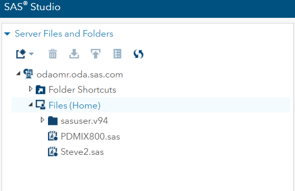
      • To do this – right click on Files(Home)
      • Select Upload Files
      • Select your file and upload

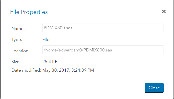
2.  Your INFILE statement will need to know where your files are located. They are not on C:\….  they are within the SAS Studio environment.  To find them, right-click on the file and select Properties

3.  Copy the information in the Location section to use for your INFILE statement.

Data trial;
    Infile “/home/edwardsm0/trial.csv” dlm=”,” firstobs=2;
Input ID$ trmt$ weight height;
Run;

Viewing the data in SAS

We’ve just imported our data and I see nothing!  What happened?  Did I do something wrong?  My log window says my data has been successfully imported, but where did the data go?

Once you’ve imported your data, SAS saved it in a dataset within its program. So think of is as a blackbox and somewhere in that blackbox is a dataset called TRIAL.  How do you go about viewing it?  Let’s use a PROCedure called PRINT.

PROC PRINT will show you your data in the Output window.

Proc print data=trial;
Run;

These statements will printout ALL the observations in your dataset.  Note when we say “printout” it prints to the screen and not to your printer.  Please note that specifying the dataset you are working with is an EXCELLENT habit to get into.  In this case we are interested in viewing the data contained in the TRIAL dataset – data=trial

To view only the first 5 observations in this dataset we can add an option at the end of the Proc print statement.

Proc print data=trial (obs=5);
Run;

Maybe we want to view observations 6-8 we can a second option at the end of our Proc print statements

Proc print data=trial (firstobs=6 obs=8);
Run;

This tells SAS that the first observation we want to view is the 6th observation of a total of 8 observations we are looking at.

We can also tell SAS that rather than looking at all the variables we only want to see TRMT by adding a var statement to our Proc print.

Proc print data=trial (obs=5);
  var TRMT;
Run;

SAS Programming/Coding TIP

1. Add comments to everything you do in SAS.  Use the *  ;  or /*  */  For example:

/*  To test whether I read my data correctly I will use the Proc Print to view the first 10 observations  */

Proc print data=trial (obs=5);
Run;

2.  ALWAYS specify the data that you are using with your PROCedure.

3.  ALWAYS add a RUN; statement at the end of your DATA step and at the end of each PROCedure.  Makes your code cleaner and allows you to select portions of your code to run.

4.  Indenting the lines of code between the PROCedure name and the RUN; statement makes it easier to read your coding.

5.  SAS is NOT case sensitive with respect to your code, however, it is with your data.

6.  The more you code in SAS, the more apt you are to develop your own coding style.