Category: Experimental Designs

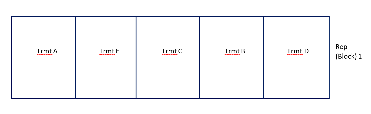
For the purposes of this workshop we will work with some fictitious data.  A trial was conducted with 10 reps (blocks), each rep was made up of 5 plots with 1 treatment applied per plot.  Treatments were randomly assigned to the 5 plots within each Rep (block).   Height of each plot was collected on 3 separate days.

The data used in this workshop can be downloaded here.  Please note that the file includes 2 years of data.  We will add the second year of data for our next analysis.

Repeated Measures Analysis

Here is the coding we will use.  I will break apart each line and explain below.

Proc glimmix data=repeated_measures plots=studentpanel;
    by year;
    class rep trmt day PlotID;
    model yield = trmt day trmt*day / ddfm=kr;
     random rep/ subject=plotID;
    random day / subject=plotID type=arh(1) residual;
Run;

Proc glimmix data=repeated_measures plots=studentpanel;

• Proc glimmix – calling on the GLIMMIX procedure to run our analysis
• data=repeated_measures – telling SAS which dataset to use – I happened to call mine repeated_measures
• plots=studentpanel – this requests all residual plots to be displayed after the analysis

    by year;

• Since we have 2 years of data – rather than breaking up the data into 2 datasets, we will ask SAS to run the analysis separately for each year – by using a BY statement inside the PROC

  class rep trmt day PlotID;

• listing out our classification variables – or the variables which tell us what group each of our observations fall into

    model yield = trmt day trmt*day / ddfm=kr;

• Our model statement
• We have an RCBD design where we have taken repeated measures on our experimental unit – the plot.  So we are interested in the trmt effect, the day effect and the interaction between then two.
• ddfm=kr – adjustment to the degrees of freedom which adjusts for bias **see  below for more information on this.

     random rep/ subject=plotID;

• Remember we have an RCBD which means we need to let SAS know that our REPs (or BLOCKs) are a random effect in our model.  Since each of our treatments only appears once in each block – there will be NO trmt*rep interaction
• This random statement tells SAS that our rep is random – we add a subject= part to the random statement to reaffirm to SAS what our experimental unit is – in this case, PlotID

    random day / subject=plotID type=arh(1) residual;

• The second random statement in this PROC – is to specify the repeated aspect of our design.
• Day is the variable which tells us where or when the measures were repeated.
• Subject tells SAS what the experimental unit was – PlotID in this case
• We also need to tell SAS what type of relationship there is between the measures taken on the experimental units is – type=arh(1).  Also known as the covariance structure.  In this example I have tried a number of them – which you should always do, and select the one which results in the model with the lowest AICC statistic.  In this example arh(1) – heterogenous autoregressive was the best fit
• residual – tells SAS that you are partitioning the R-side of the error (experimental error) into a portion due to the repeated measures taken within an experimental unit.

The output for this analysis can be downloaded here.  Start from the bottom of the output file for 1 year to review the residuals.  Please note that there are NO normality statistics produced only the plots.  To run the normality statistics you will still need to save the residuals in a new dataset and rung the PROC UNIVARIATE normal with the residuals.  However, reviewing these plots gives you a great starting point.

Once you are “happy” with the residuals, start reviewing the output from the beginning of the PROC GLIMMIX.  Carefully review the Dimensions table:

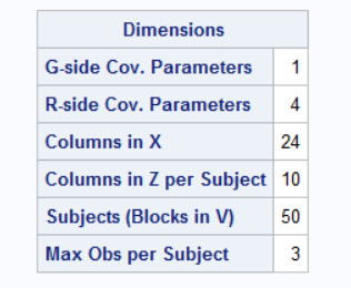
• G-side Cov. Parameters = 1 – this refers to the random effect of Rep (Block).  Remember G-side is the random variation between our experimental units.
• R-side Cov. Parameters = 4 – this refers to the random effects within our experimental units – 3 days + residual error
• Columns in X – how many levels do we have for our fixed effects in our model?  Trmt = 5, Day = 3, Trmt*day = 15, 1 for the overall mean = 24
• Columns in Z per Subject – our Rep is our random effect and we have 10 reps
• Subjects (Blocks in V) = 50 – 10 Reps with 5 plots/rep = 50 experimental units
• Max Obs per Subject = 3 – each experimental unit (plot) was measured 3 times

You should always be able to track back all these pieces of information to your model.  If you are analyzing a repeated measures it is important to ensure that the last 2 lines of this table is correct.  If they are not, then your model is not reflecting a repeated measures analysis of your trial.

Review the second year of this output to ensure it was run correctly as well.

Doubly Repeated Measures – PROC MIXED

So now let’s add in that second year.  We have a trial which was conducted 2 years in a row.  The previous analysis conducted a repeated measures on the data collected each year as a separate analysis and really as a separate trial.  But, we know there is some relationship between the 2 years, since the same location was used and the same treatments, the same experimental units – so there must be a relationship and we must account for it somehow.

There are 2 ways to handle this at the moment in SAS.  The first way we will look at is treated it as a truly doubly repeated measures – if you think about it – we have the days repeated and we have the years repeated.  Now GLIMMIX cannot necessarily handle this IF there are 2 covariance structures that need to be used – One for Year and one for day, but MIXED can – by using a Kronecker product covariance structure.

Proc mixed data=repeated_measures covtest;
    class rep trmt day PlotID year; 
    model height = trmt day trmt*day Year year*trmt year*day year*trmt*day/       ddfm=kr;
    random rep / subject=plotID;
    repeated year day / subject=plotID type=un@cs;
    lsmeans year*day;
    ods output lsmeans=lsm;
Run;

Proc mixed data=repeated_measures covtest;
    class rep trmt day PlotID year; 

• These are the same as our PROC GLIMMIX above with the addition of our Year effect in the CLASS statement

model height = trmt day trmt*day Year year*trmt year*day year*trmt*day/       ddfm=kr;

• Our model has now been expanded to include the effect of the Year.  We are interested in the main effect of Year, the interaction between year and trmt, the interaction between year and day, and the three-way interaction of year, trmt, and day.  If you think these through you will see that we are indeed interested in the if and how the different years have affected the trmt and the day repeated aspect of our trial.
• Note that we are treating YEAR as a fixed effect.

  random rep / subject=plotID;

• same as our GLIMMIX statements above

  repeated year day / subject=plotID type=un@cs;

• MIXED has a specific REPEATED statement whereas GLIMMIX no longer has this.  Note that the structure of this statement is almost identical to the RANDOM statement we used in GLIMMIX with two changes:
  • There is no need to say RESIDUAL with the REPEATED statement in MIXED
  • We are telling MIXED that we have 2 covariance structures with the type= statement
  • un@cs – tells SAS that we want it to use an UNstructure covariance structure for the 2 years, and a CS(compound symmetry) structure for the 3 day measurements.

  lsmeans year*day;
    ods output lsmeans=lsm;

• These statements are built the same in MIXED and GLIMMIX – I added them here so we can review the lsmeans

To review the complete output provided by this code, please download and view the PDF file.

Doubly Repeated Measures – PROC GLIMMIX

So as I mentioned earlier GLIMMIX cannot handle the true doubly repeated aspect of some of our experiments – what it cannot do is recognize and implement the 2 difference covariance structures for the 2 repeated effects.  However, what we can do is add YEAR as a random effect into a GLIMMIX and our fixed effect results are similar.

Proc glimmix data=repeated_measures plots=studentpanel nobound;
    class year rep trmt day PlotID;
    model height = trmt day trmt*day Year year*trmt year*day year*trmt*day/ ddfm=kr;
    random rep/ subject=plotID group=year;
    random day / subject=plotID type=cs residual;
    lsmestimate year*trmt “2016 Treatments AandB vs C” -1 -1 2 0 0 0 0 0 0 0 ;
    lsmestimate year*trmt “2016 vs 2017 Treatment A” -1 0 0 0 0 1 0 0 0 0 ;
Run;

Proc glimmix data=repeated_measures plots=studentpanel nobound;
    class year rep trmt day PlotID;
    model height = trmt day trmt*day Year year*trmt year*day year*trmt*day/ ddfm=kr;

• These statements are the same as the previous GLIMMIX and/or MIXED.  Only difference is that I added the nobound option to allow our random effects to have negative variance.  Everything else is the same!

    random rep/ subject=plotID group=year;

• This statement tells SAS that our REP is random – we have seen this above in both the GLIMMIX and MIXED coding.
• But this time we have added a GROUP=option.  This allows us to group the random REP effect within each year.  Essentially adding a rep(year) effect to our model.

    random day / subject=plotID type=cs residual;

• This is our repeated statement for day – which we have seen already.

    lsmestimate year*trmt “2016 Treatments AandB vs C” -1 -1 2 0 0 0 0 0 0 0 ;
    lsmestimate year*trmt “2016 vs 2017 Treatment A” -1 0 0 0 0 1 0 0 0 0 ;

• Another new statement that you should be aware of.  The LSMESTIMATE allows us to essentially run contrasts amongst our LSMeans – something we were unable to do with MIXED.
• Something to consider for future analyses and research questions

To review the complete output provided by this code, please download and view the PDF file.

GLIMMIX – Random rep/ group=year VS Random rep(year)

I mentioned above that the statement  random rep/ subject=plotID group=year;  was similar to adding the rep(year) effect as a random effect.  To show you the differences between the output try running the following code:

Proc glimmix data=repeated_measures plots=studentpanel nobound;
    class year rep trmt day PlotID;
    model height = trmt day trmt*day Year year*trmt year*day year*trmt*day/ ddfm=kr;
    random rep(year)/ subject=plotID ;
    random day / subject=plotID type=cs residual;
    lsmestimate year*trmt “2016 Treatments AandB vs C” -1 -1 2 0 0 0 0 0 0 0 ;
    lsmestimate year*trmt “2016 vs 2017 Treatment A” -1 0 0 0 0 1 0 0 0 0 ;
Run;

random rep(year)/ subject=plotID ;

• This is the only line that is different.  Similar to above – we are adding the random effect of rep(year), and reminding SAS that our experimental unit is plotID but specifying this as the subject

Differences in the output of the 2 previous analyses:

1. random rep/subject=plotID group= year;  provides 2 G-side covariance parameters – one for each year.  Whereas the random rep(year) / subject=plotID; only provides one parameter the rep(year) effect
2. AICC for the group=year model = 1638.32, whereas the AICC for the rep(year) model =1656.04.  Suggesting that we are doing a better job with the group=year model.
3. Since we have different number of covariance parameters, we will have different estimates:
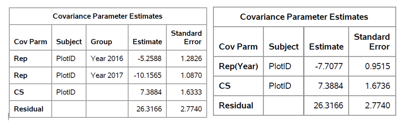
4. Overall the Type III Fixed effects for the 2 models were identical

DDFM=KR

We see this added to many of our models and let’s be honest, we ask ourselves WHY?  Is this something I should be adding or not?  When should I be using this?

A quick review

Mixed methods were developed in the 1980-1990s and there has been a lot of research surrounding these methods.  Especially surrounding the are of small sample sizes – now this is a relative term and I will not provide any thoughts as to what is referred to by small sample sizes.

Research has found that when estimated variance and covariance parameters are used to calculate statistics, such as the F-statistic, the results are often biased upward, while the standard error estimates used to calculate confidence intervals are often biased in the opposite direction or downwards.  What does this mean?  We have a higher F-statistic – greater chance of seeing differences, and a small confidence interval.  Now these trends tend to happen when we use mixed methods – which most of us are today.

Research has shown the following trends:

• There is NO problem when we have balanced designs with a FIXED effects model
• There is a slight problem with we have unbalanced designs with a FIXED effects model
• A BIG problem when we have more complex models

So, we can play it safe and use the DDFM adjustment for all of our models.  Let’s be honest, we may have small sample sizes, and we may never be sure whether our model is one that is considered complex or not.

It has been recommended that adding the DDFM=KR should be something that becomes second nature to us and should be added to all of our MODEL statements in GLIMMIX.

Split plot and strip plot (or split block) designs are commonly used in the agronomy, however, they don’t stop there.  We quite often have limited resources and may add on a factor or two on top of our current trial.  This blog post and session will expand on the Split-plot and the Strip-plot (split-block) designs.

Split-split-plot

We have 3 experimental units with 3 differing sizes.  The whole plot, the sub-plot, and the sub-sub-plot.  This link contains a PDF document that displays the Split-split plot design and also contains the Statistical model.

Factor A is the Whole plot – with two levels: A1 and A2.  A1 and A2 are randomly assigned within a block (or rep).  In this illustration we have 2 Blocks (Reps).

The WHOLE plot is now divided into SUB Plots.  Factor B, which has 3 levels is randomly assigned to each level of Factor A in the WHOLE plots.

The SUB plot is now divided into SUB-SUB Plots.  Factor C, which has 5 levels is randomly assigned to each level of Factor B in the SUB plots.

Let’s build the model for the Split-Split plot design as modeled above:

Split-split-split plot

An extension of the split-split-plot, with a 4th experimental unit.  Same as above 4 differing experimental unit sizes, and therefore 4 errors to be aware of.

Split-plot x Split-block (strip-plot)

The combinations do not seem to end.  The more we look into these designs, the more I realize that many trials that we currently conduct may not be what we think they are.

In this case we are looking at the Split-block or Strip-plot design and within each row/column combination we are adding a third factor within this experimental unit and will aim to randomly assign them – leading us to a Split-plot x split-block design.

I will update with a picture of a design and the statistical model that accompanies it.

 

Conclusion

After working through these three examples, which design do you think you truly have?

I propose for the last workshop session in April, that we review Latin Square designs, and the combination of Split-plot and latin squares, as I suspect this will talk to a few researchers 🙂

What is an experimental design?

Is the process of planning a study to meet specified objectives.  An experiment that SHOULD be designed to match a specific research question.

Steps to designing an experiment

1. Define the EXPERIMENTAL UNIT
   What is the difference between an EXPERIMENTAL UNIT and a SAMPLING UNIT?
2. Identify the types of variables
3. Define the treatment structure
4. Design the design structure

Experimental Unit  vs. Sampling Unit

Experimental unit is the unit to which the treatment is applied to.

Sampling unit is a fraction of the experimental unit.

Examples of potential experimental units:

• An animal
• A cage with 5 birds inside
• A plot in a field
• A box of fruit
• A tree
• A pot of plants
• A growth chamber
• A fish tank
• A tray of seedlings
• A taste panelist
• A sample of a new food product
• A bench in a greenhouse

Examples of potential sampling units:

• 1 bird in a cage
• A quadrant in a plot of a field
• 5 apples from a box
• A branch or leaf of a tree
• 1 plant from a pot of plants
• A tray or shelf placed in a growth chamber
• An individual fish from a fish tank
• One pod of seedlings from a tray
• A plot on a bench in a greenhouse

Experimental Error

Measure of the variation that exists among observations taken on the experimental units that are treated alike.

Sources of Experimental Error

1. Natural variation among experimental units
2. Variability of the measurements taken (response)
3. Inability to reproduce the treatment conditions exactly from one unit to another
4. Interaction between the treatments and the experimental units
5. Any other extraneous factors that may influence the response

With any statistical analyses, what we are looking for is an estimate of the variation of the experimental error.  So, the variation between our experimental units – We need this  to test treatment differences.

Variation of observations within an experimental unit will not give us treatment differences!

Completely Randomized Design (CRD)

Treatments that are randomly assigned to experimental units.

Experimental unit is the individual plot/square in the design.  The statistical model is represented by:

Where:

Yij = Observation on the jth experimental unit on the ith treatment
μ = overall mean
τi = the effect of the ith treatment
εij = experimental error or residual

The experimental error is variation among experimental units on the same treatment. The unexplained variation – the residual – what’s left.

Randomized Complete Block Design (RCBD)

In any experiment we conduct, we have experimental error.  Our goal is to take control over our experimental error so we can study the effects of our treatments.  Blocking is one way to take control of our experimental error.

Blocking occurs when we group experimental units in a way where the variation of the experimental units within the blocks is less than the variation among all the units before blocking.

Each block highlighted as the different colours or the columns in the above table.  Within each block all the treatments will appear an equal amount of time.  The statistical model would be:

What happens though when we have more than one experimental unit/treatment in each block?  If you look at the current design – you have one measurement per treatment in each block – so there is not enough measures to see whether the treatments are doing something different across the blocks.  But when we have more than one experimental unit per treatments in a block, then you have variation to examine.  So your model would now be:

Split Plot Design

A design where you have 2-3 factors or treatments of interest, yet the experimental units of each treatment are different sizes.

What are the 2 sources of experimental error?

Variation between the Blocks where A was assigned.  Two blocks have the A1 treatment and two blocks have the A2 treatment.  The main plot is the A treatment.

The second source of experimental error is the variation among the experimental units.  The subplot is the B treatment.  The statistical model is:

Split Block or Strip-plot

Two treatments that are applied as a strip as an example.  Here is one block

If we are interested in looking at the effect of Treatment A – what is the correct error term?  Start by asking yourself what is the experimental unit for treatment A?  Then think about the definition of experimental error – variation between experimental units that were treated the same….

What about Treatment B?

And the interaction between Treatment A and Treatment B?

The statistical model is:

Let’s see how much we can get through.