Category: GLIMMIX

As we begin to appreciate the various types of data we collect during our research and understand that we should be acknowledging their diversity and taking advantage of this, we find ourselves working with binary and multinomial data quite often.  These types of data also lead us to working with Odds Ratios more than…  maybe we want to 🙂

I’ll be the first to admit that if there was a way to avoid them – I would – they can be a challenge to interpret and fun to play with – all at the same time!

So in an attempt to help interpret these OR (odds ratio) I’m going to lay out the steps you’ll need.  I’m also going to use the SAS output as a guide.  It really doesn’t matter what software you use to obtain your results (maybe I’ll play with R later this summer and add to this post), the steps will be the same.

So let’s start with some data – I’ve created a small Excel worksheet that contains 36 observations.  Each observation was assigned to 1 of 4 treatments and has a measure for a variable called Check (0 or 1) and a variable called Score (1, 2, 3, 4, 5).  Check is a binary variable whereas Score is a multinomial ordinal variable.

The goal of this analysis was to determine whether there was a treatment effect for both the Check and Score variables.  I will list the SAS code I used in each section.  But, to start let’s try this out:

Proc freq data=orplay;
    table trmt*check trmt*score;
    title “Frequencies of Check and Score for each Treatment Group”;
Run;

I like to use PROC FREQ as a starting point to help me get familiar with my data – give me a sense as to how many observations has ‘0’ or ‘1’ for each treatment group for the CHECK variable and a similar view for the SCORE variable.

Binary Outcome Variable – CHECK = 0 or 1

I then ran the analysis for my CHECK variable:

Proc glimmix data=orplay;
    class trmt;
    model check = trmt / dist=binary link = logit oddsratio(diff=all) solution;
    title “Results for Check – in relation to the value of ‘0’ in Check”;
    contrast “Treatment A vs Treatment B” trmt -1 1 0 0 ;
    contrast “Treatment A vs Treatment C” trmt -1 0 1 0 ;
    contrast “Treatment A vs Treatment D” trmt -1 0 0 1 ;
    contrast “Treatment B vs Treatment C” trmt 0 -1 1 0 ;
    contrast “Treatment C vs Treatment D” trmt 0 -1 0 1 ;
    contrast “Treatment C vs Treatment D” trmt 0 0 -1 1 ;
Run;

The first time I ran this code – I noticed that it is creating the results in relation to the value of ‘0’ for my CHECK variable.  The output states: “The GLIMMIX procedure is modeling the probability that CHECK = ‘0’ ”  This is ok!  But, if you are studying the response to your treatments and the response you are interested in is the ‘1’ – then let’s add a bit to the SAS coding to obtain the results in relation to CHECK = ‘1’.  This change will depend on what you are studying – when we start talking about Odds Ratios – we will be saying that the Odds of CHECK = 1 are ….  or the Odds or CHECK=0 are ….

So my new coding will be:

Proc glimmix data=orplay;
    class trmt; 
    model check (event=”1″) = trmt / dist=binary link = logit oddsratio(diff=all) solution;
    title “Results for Check – in relation to the value of ‘1’ in Check”;
    contrast “Treatment A vs Treatment B” trmt -1 1 0 0 ;
    contrast “Treatment A vs Treatment C” trmt -1 0 1 0 ;
    contrast “Treatment A vs Treatment D” trmt -1 0 0 1 ;
    contrast “Treatment B vs Treatment C” trmt 0 -1 1 0 ;
    contrast “Treatment C vs Treatment D” trmt 0 -1 0 1 ;
    contrast “Treatment C vs Treatment D” trmt 0 0 -1 1 ;
Run;

Take note of some of the coding options I’ve used.  At the end of the MODEL statement I’ve asked for the odds ratios and the differences between all of them, as well as the solutions to the effects of each treatment level.  Also note that I have also requested the CONTRASTS between each treatment effect.  All of these pieces of information will help you to tell the story about your CHECK variable – but remember we chose to talk about CHECK=1.

The output can be viewed at this link – output_20190625– be sure to scroll to the appropriate section – entitled “Results for Check – in relation to the value of ‘1’ ”

The Parameter Estimates table provides the individual estimates of each treatment.  Note that the last treatment has been set to 0 – which allows us to view how each treatment compares to the last.  Also note the t Value and associated p-value.  This will help you decide whether the estimate differs from 0 or not.  As an example – Trmt A has an estimate of 2.7726 and is different from 0.  Leading us to suggest that the effect of Trmt A is 2.77 times greater than that of Trmt D.  Trmt B on the other hand does not differ from 0 and therefore provides similar results as Trmt D.

The next table our Type III fixed effects – suggests that there may be a treatment effect – although the p-value = 0.0598 – so I will leave that up to the individual reader to interpret this value.  Personally, I will not ignore these results based solely on a p-value > than the “magical” 0.05.

Moving onto the next table – Odds Ratio Estimates.  The FUN one!!!  So – the first thing to keep in mind – please look at the 95% Confidence Limits first!  IF the value of ‘1’ is included in the range – this means that the odds are equal for a CHECK =1 for the 2 treatment groups listed.  So… let’s try it.

From the table we see:

Trmt A vs Trmt B  Odds ratio estimate = 0.250 95% CI ranges from 0.033 – 1.917

The odds of having a Check = 1 are the same for observations taken from Trmt A or Trmt B.  This is due to the fact that the CI range includes 1 – equal odds.

Trmt A vs Trmt D Odds ratio estimate = 0.063 95% CI ranges from 0.005-0.839

The odds of having a Check = 1 are 0.063 times less for observations on Trmt A than Trmt D.

The trick to reading these or best practices:

1. Check the CI first – if ‘1’ is included – then there are no differences and you have equal odds or equal chances of the event happening – or in this case of having CHECK=1 in either treatment.
2. If ‘1’ is not included in the CI – then we have to interpret the Odds Ratio estimate.
3. Always read from Left to Right for the treatments – so the Treatment on the left has a BLANK odd over the Treatment on the right.
4. Now the value of the odds ratio estimate tells you whether it is greater or less than.  If the value of the estimate is < 1 then we say the odds of Check = 1 is less for the Treatment group on the left than the Treatment group on the right.
5. If the value of the estimate is > 1 then we say the odds of Check = 1 is greater for the Treatment group on the left than the Treatment group on the right.
6. ALWAYS start with the odds of X happening – so in this case that Check =1.

Let’s go back and look at the results for CHECK = 0.  If you go back to the Results PDF file and scroll up to the section titled:  “Results for Check – in relation to the value of ‘0’”.

From the Odds Ratio Estimates table we see:

Trmt A vs Trmt B  Odds ratio estimate = 4.000 95% CI ranges from 0.522 – 30.688

The odds of having a Check = 0 are the same for observations taken from Trmt A or Trmt B.  This is due to the fact that the CI range includes 1.

Trmt A vs Trmt D Odds ratio estimate = 16.000 95% CI ranges from 1.192 – 214.687

The odds of having a Check = 0 are 16 times greater for observations on Trmt A than Trmt D.

I hope you can see how the statements are saying the same thing – but we just have a different perspective.  These can get tricky – but just keep in mind – what the outcome is – CHECK = 1 or CHECK = 0 – start by saying this first and then add the less or greater chance part after.

Multinomial Ordinal Outcome Variable

Most often we work with data that has several levels, such as Body Condition Score (BCS) in the animal world, or Disease severity Scores in the plant world.  Any measure that is categorical in nature and has an order to is – should be analyzed as a multinomial ordinal variable.

Guess what?  When you work with this type of data – you are back to working with Odds Ratios but this time you have several levels and not the basic Y/N or 0/1.  So how do we work with this?  How do we interpret these results?

In the Excel spreadsheet I provided above there was a second outcome measure called SCORE – this is a score or ordinal outcome variable with levels of 1 through to 5.  The SAS code I used to analyze this variable is as follows:
Proc glimmix data=orplay;
    class trmt; 
    model score = trmt / dist=multi link=cumlogit oddsratio(diff=all) solution;
    title “Results for Score – a multinomial outcome measure”; 
    estimate “score 1: Treatment A” intercept 1 0 0 0 trmt 1 0 0 0 /ilink;
    estimate “score 1,2: Treatment A” intercept 0 1 0 0 trmt 1 0 0 0 /ilink;
    estimate “score 1,2,3: Treatment A” intercept 0 0 1 0 trmt 1 0 0 0 /ilink;
    estimate “score 1,2,3,4: Treatment A” intercept 0 0 0 1 trmt 1 0 0 0 /ilink;
    estimate “score 1: Treatment B” intercept 1 0 0 0 trmt 0 1 0 0 /ilink;
    estimate “score 1,2: Treatment B” intercept 0 1 0 0 trmt 0 1 0 0 /ilink;
    estimate “score 1,2,3: Treatment B” intercept 0 0 1 0 trmt 0 1 0 0 /ilink;
    estimate “score 1,2,3,4: Treatment B” intercept 0 0 0 1 trmt 0 1 0 0 /ilink;
    estimate “score 1: Treatment C” intercept 1 0 0 0 trmt 0 0 1 0 /ilink;
    estimate “score 1,2: Treatment C” intercept 0 1 0 0 trmt 0 0 1 0 /ilink;
    estimate “score 1,2,3: Treatment C” intercept 0 0 1 0 trmt 0 0 1 0 /ilink;
    estimate “score 1,2,3,4: Treatment C” intercept 0 0 0 1 trmt 0 0 1 0 /ilink;
    estimate “score 1: Treatment D” intercept 1 0 0 0 trmt 0 0 0 1 /ilink;
    estimate “score 1,2: Treatment D” intercept 0 1 0 0 trmt 0 0 0 1 /ilink;
    estimate “score 1,2,3: Treatment D” intercept 0 0 1 0 trmt 0 0 0 1 /ilink;
    estimate “score 1,2,3,4: Treatment D” intercept 0 0 0 1 trmt 0 0 0 1 /ilink;
Run;

Notice the changes in the MODEL statement from the example listed above?  We have a distribution listed as multi(nomial) and we are using the cumlogit link.  I have also included the oddsratio(diff=all) and solution options – just as we did above.  I’ll talk about all those estimate statements after we review how to read the odds ratios.

If you go back to review the PDF results file from above or here – please scroll down to the last analysis titled ” Results for Score – a multinomial ordinal measure”.

First thing to note is the information listed on the Response Profile Table:

The note at the bottom of this table is the KEY to reading and interpreting the Odds Ratio.  We are modelling the probabilities of have a lower score!  That’s what this means!  So when we are talking about the OR – we are always talking about the odds of having a lower SCORE.

So let’s jump down a bit in the output file.  The Type III Fixed Effects table is telling us that there are some differences present.

Now let’s look at the Odds Ratio Estimates table – using the same best practices as listed above – let’s try the reading the same 2 comparisons we did above:

From the Odds Ratio Estimates table we see:

Trmt A vs Trmt B  Odds ratio estimate = 0.578 95% CI ranges from 0.090 – 3.708

The odds of having a lower SCORE are the same for observations taken from Trmt A or Trmt B.  This is due to the fact that the CI range includes 1.

Trmt A vs Trmt D  Odds ratio estimate = 54.544 95% CI ranges from 5.280 – 563.489

The odds of having a lower SCORE are 54.54 times greater with Treatment A than with Treatment D.

Seems pretty easy right?  If you keep these guides in your mind – it will be easy to read the results.  The tricky part is what are those scores?  Is a lower score or a higher score better?  Trust me – you can get pretty twisted up when you are looking for a higher score, but the results are referring to a lower score – oh my!!

Ways to work with this – you can change the order of your data – sorry there is no SAS coding as in the 0/1 data.

Alright – let’s keep working through the output.  I added quite a few ESTIMATE statements.  These provide us with the cumulative probabilities of obtaining a particular Score in a particular treatment.  Hmmm…  this might be the answer to interpreting the odds Ratios???  Remember – it all comes back to your Research Question!!

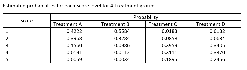
Estimated Probabilities for each Score level

Let’s take a look at the Estimates table – you should see a list that matches all the ESTIMATE statements I listed in the SAS code.  Each statement is calculating the estimated probabilities for a given Treatment and Score levels.  For example:

estimate “score 1: Treatment A” intercept 1 0 0 0 trmt 1 0 0 0 /ilink;

Will provide us with the estimated probability that an observation in Treatment A will have a Score of 1.  In the Estimates table the column Mean provides us with that probability.  In this example, we have a value of 0.6383 – so with this dataset, there is a 63.83% probability that an observation on Treatment A will have a Score value of 1.

Remember these are cumulative probabilities – so to calculate the probability of have a Score of 2 in Treatment A – we take the value for the second Estimate statement which states:

estimate “score 1,2: Treatment A” intercept 0 1 0 0 trmt 1 0 0 0 /ilink;

This statement shows the probability of having a score of 1 and 2 for Treatment A which has a value of 0.8190.  Therefore, to obtain the estimated probability of having a Score of 2 in Treatment A we would need to subtract the probability of having a Score = 1 – which would be:  0.8190 – 0.6383 which equals 0.3968 or 39.68% chance of having a Score of 2 in Treatment A.

You would follow the same process to obtain the estimated probabilities for Score of 3 and 4.  Since we have 5 Scores – the last last would be calculated as 1 – cumulative probability for Scores 1, 2, 3, 4.  In this example – we would have 1 – 0.9941 = 0.0059 or 0.59% chance of having a Score of 5 with Treatment A.

If you were to calculate all the estimated probabilities for this example you would have a table similar to this:

Conclusion

Working with binary and multinomial ordinal data can be fun and challenging.  Just remember – if the Confidence Interval includes the number 1 – then the two treatments have equal odds of happening.

To read the Odds ratios – The odds of having a lower score OR having a Check =1 are X greater  (if the value is >1) or X less  (if the value is <1) for the treatment on the left compared to the treatment on the right.

I hope this helps!  I’ll keep working on better ways to explain this.