SAS Workshop: Introduction and Getting the data in

PDF version of Notes

Available Versions of SAS

  • PC Standalone Version – PC-SAS
    • Available for Windows ONLY – if you’re using a Mac, you will need to have a VM to emulate Windows to run this version
    • Available through CCS Software Distribution Centre – $118.63 for a new license and $75/year renewal license. This information was downloaded on May 29, 2017, please check https://guelph.onthehub.com/WebStore/Welcome.aspx for updated pricing and access information or email 58888help@uoguelph.ca for more information
  • Animal Biosciences department ONLY
    • Access the server version of PC-SAS
  • SAS University Edition
    • This is free for all academics to use. You can download the free version from https://www.sas.com/en_ca/software/university-edition.html
    • This is available for both Mac and Windows users
    • Please note, that you will be required to update this version every year.  SAS will send you a reminder notice, approximately 1 year from your installation date.
  • SAS OnDemand
    • This is also free for academics
    • This is SAS’ in the cloud version of the University Edition
    • Environment is the same as the University Edition, the difference is that you are using the SAS service in the Cloud, all your files are stored in the Cloud and not on your local system, and you are using their computer resources NOT your own system – accessed through a web browser with your own personal login

What Parts of SAS do you have access to?

SAS is an extremely large and complex software program with many different components.  We primarily use Base SAS, SAS/STAT, SAS/ACCESS, and maybe bits and pieces of other components such as SAS/IML.

SAS University Edition and SAS OnDemand both use SAS Studio.  SAS Studio is an interface to the SAS program and contains the following components:

  • BaseSAS – base SAS programming, DATA Step
  • SAS/STAT – the PROCs used for statistical analyses
  • SAS/IML – SAS’ matrix programming language
  • SAS/ACCESS – allows you to interact with different data formats
  • Some parts of SAS/ETS – time series analysis

If you are using the PC or Server SAS versions, you may have access to more than the modules listed above.  To see exactly what you have access to, you can run the following code:

Proc Setinit;
Run;

You will see the components available to you listed in the log window.

SAS_setinit_log_window_results.png

Also note the additional information available to you:

  • License information
  • Expiration date – very handy to be aware of, especially if you are running your own copy of your PC
  • SAS components available to you

What does SAS look like?

There are a number of components to the SAS interface:

  • Results and Explorer windows to the left
  • Editor, Log, Output, and Results Viewer windows to the right, taking up most of the screen

SAS_Windows_interface_Contents_window_Editor_Log_Windows.jpg

What do each of these windows do?

  • Results Window –  a Table of Contents for all of your results.
  • Explorer Window – similar to Windows Explorer – allows you to navigate SAS libraries and files
  • Editor Window – this is where you will spend most of your time, writing and editing program files
  • Log Window – this window is extremely helpful, think of it as your best friend in SAS, it tells you what SAS has done every step of your program and processing
  • Output Window – SAS versions 9.2 and earlier, use this window to display all results and output.  SAS 9.3 and higher use a new window called the Results Viewer.  All the results are presented in an HTML format.

How does SAS work?

SAS is divided into 2 areas:

  • DATA step
  • PROCs (short for PROCedures)

DATA step is all about data manipulation – one of the key strengths to SAS
PROCs – this is where you will find most of your statistical procedures.

How do you get data into SAS?

The primary reason we use SAS is to perform statistical analyses on some data.  However, we need to ensure that the data we have collected is brought into SAS correctly.  I’m sure you’ve heard of “garbage in, garbage out”?  This cannot be more truer than when you collect data and bring it into a statistical package.

There are different ways to bring data into SAS.  I will try to review and provide my thoughts on 3 different ways I see my students performing this task.  However, before we import data into any software package, we need to ensure the data is “clean” and in a format that will be accepted into the package.  So let’s talk about the most common way researchers enter their data – EXCEL.

Using Excel to enter data and Statistical Software packages

Most people use Excel to enter their data and that’s great!  The look of it is neat, ordered and we can do quick summaries, such as means and sums.  We can also make Excel look pretty by adding colours, headings, footnotes, or maybe notes about what we did and how.  In the end, Excel can be a very versatile tool.  But, we need to keep in mind that Excel is NOT a statistical package and that we are using it to collect our data.  That being said, I recognize many people use it for more than it was set out to be.

Let’s take a look at an example of how Excel is used.

2018 Trial Data

Everyone uses Excel differently when entering data.  This file is a very simple example.  Many people will highlight cells or add comments, etc…  Every file will need to be “cleaned” before it can be used in SAS.  These are recommended steps to clean any Excel file.

Recommended steps to clean an Excel file:

  • Copy the entire sheet into a blank worksheet.  This allows you to keep the formatted version while working on a clean version.
  • Label the new worksheet SAS or something that makes sense to you.  This way when we import the data you will know which worksheet contains the clean data.
  • Remove all the formatting.  In Excel, Click on the CLEAR button and select Clear Formats.  This will remove all Excel formatting from the worksheet.
  • The top row of the Excel file needs to contain the name of the variables you wish to use in SAS.  Note that some files may have titles and/or long descriptions at the top of the worksheet.  These need to be deleted.
  • The top row of the Excel file needs to contain the name of the variables you wish to use in SAS.  You may need to modify the headings of the columns.
  • The variable names are ones that will have a significance to you.  Please DOCUMENT these changes so you know what is contained in your dataset!  I will provide more information on Variable Labels and Value Labels in a follow-up post
  • Don’t forget to save your Excel file!
  • If there are any notes at the bottom of your worksheet or anywhere else in the worksheet – you will need to delete these.

RECAP:

  1. Copy data into new worksheet
  2. Rename worksheet for easy identification later
  3. Clean variable names in the first row
  4. Second row contains your data and NOT blanks

TIPS:

SAS naming conventions:

  • variable names do not contain any “funny” characters such as *, %, $, etc…
  • variable names begin with a letter
  • variable names may contain a number, but cannot begin with a number
  • NO spaces allowed!  You may use _ in place of a space

IMPORTING EXCEL FILES INTO SAS – works best with individual PC-SAS license

Using the IMPORT feature in SAS is probably the easiest way of bringing data into the SAS program.  To import the data follow these steps:

  1. In the SAS program – File -> Import Data
  2. You will now answer each step of the Import Wizard.
  3. With SAS 9.2, you will need to save your Excel files as the older 97-2003 .xls format.  This version of SAS does NOT recognize the .xlsx ending for Excel
  4. Browse your computer to find and select your Excel file
  5. Select the worksheet in the file using the dropdown box in SAS.  This is why I suggested earlier to call it SAS or something you will remember
  6. This next step can be tricky.  Leave the Library setting to WORK.  In the Member box provide SAS with a name for your datafile to be saved in SAS.  For this example let’s call it TRIAL
  7. The next step is optional!  If you are planning on importing more files that have the same structure or where your answers to the Wizard will be the same, this step allows you to save the program (or syntax) that SAS creates to import the file.
  8. Finish and your file is now in SAS
  9. Check the Log Window


COPY AND PASTE DATA INTO SAS

As much as I would like to discourage people from using this method of bringing data into SAS, it is a viable option about 95% of the time.  In most cases this method will work, however there is the odd case, about 5% of the time where this method will fail.

Let’s work through how we enter data into Excel and translate our steps into SAS

First thing most of use do when entering data into Excel is to create variable names or headings in the first row of Excel.  We then begin to type our data in the second row.  When we’ve completed entering the data or we have a page full of data, that’s when most of us remember to save the file.  Sound familiar?

In SAS we can do all of these steps using a DATA Step.  We will be creating a program or writing syntax in the SAS editor for this bit.  To start, SAS likes us to save our file FIRST, before we enter any data – contrary to what we traditionally do in Excel.  We start our program.

Data trial;

The first thing we did in Excel was label our columns – this is the second line of our SAS code:

Data trial;
Input ID trmt weight height;

The next thing we do in Excel is start entering our data.  In SAS, we first let SAS know that the data is coming by adding a datalines; statement in our code and then we enter our data.

Data trial;
Input ID trmt weight height;

Datalines;
13K Pasture 89 47

In order to complete our data entry in SAS, we need to let SAS know that there are no more data points and to go ahead and save the file.  To do this we add a “;” all by itself at the end of the data and a Run; to let SAS finish the data and save the file.

Data trial;
Input ID trmt weight height;
Datalines;
13K Pasture 89 47
;
Run;

When you run this code – you will receive a number of errors.  SAS loves numbers and the data we are trying to read in has letters and words in it.  We need to let SAS know that the variables we’ve called ID and trmt, are not numbers.  We do this by adding a $ after the variable names.

Data trial;
Input ID$ trmt$ weight height;
Datalines;
13K Pasture 89 47
;
Run;

Now that should work without any errors in the LOG window.

Rather than retyping all the data, we can copy it from Excel and paste it after the datalines statement.  As I noted above, this will work most of the time, but there are times where it does not work.  Why you may ask?  I suspect it is some hidden Excel formatting that plays havoc with SAS, but I cannot identify exactly what it is.  Just note that this method may fail at times.

READING DATA FROM A FILE

In order to read data that has been saved to a file, the INFILE statement must be used before the INPUT statement.   Think of it in these terms.  You need to tell SAS where the data is first (INFILE) before you can tell it what is contained inside the file (INPUT).  Another trick to remembering the order, the two statements are to be used in alphabetical order.

NOTE: Before we can read in a datafile into SAS, we need to save it in the proper format from Excel.  On a WINDOWS laptop/computer, in Excel, please select File -> Save As -> Save as type should be CSV(Comma Delimited).  On a Mac, in Excel, please select File -> Save As -> Type should be MS-DOS Comma Delimited.

Once you have a datafile that has been created in Excel or another program, and if that file is a text file, which means a file that only has data and spaces, then the INFILE statement will be only be used to tell SAS the location of the text file on the computer. Here is an example:

Data trial;
Infile “C:\Users\edwardsm\Documents\Workshops\SAS\trial.csv”;
Input ID$ trmt$ weight height;
Run;

A Comma Separated Values(CSV or Comma Delimited) File is one of the most common text files used for data today, probably more common than a text file.  If you use a text file, we assume that there are only empty spaces between the variable values.  With a CSV file there are commas (,) separating the values, so we need to tell SAS this.  This can be done by adding DLM (which is short for DELIMITER) = “,” at the end of the INFILE statement.

There is another aspect of our CSV files that we will need to tell SAS about.  When we are working in EXCEL and create our CSV files, we use the top row to list our variable names (to identify the variables).  This is fine, but again, we need to let SAS know that we don’t want it to start reading the data until the second row or whichever row your data starts in.  We do this by adding FIRSTOBS=2 at the end of the INFILE statement.  So we will have something that looks like this:

Data trial;
Infile “C:\Users\edwardsm\Documents\Workshops\SAS\trial.csv” dlm=”,”      firstobs=2;
Input ID$ trmt$ weight height;
Run;

With a CSV file, remember that we are using a “,” to separate the variable values or the columns that were in Excel.  What happens though, if we have commas in our data?  For example, instead of Chocolate cookies, we may have entered the data to show Cookies, chocolate.  If we leave the INFILE statement as it reads now, when SAS encounters one of those commas, it will move onto reading the next variable, which we know will fail or make a mess of our data.  To prevent this from happening we need to add the DSD option at the end of our INFILE statement.

And…  0ne last note about using the INFILE statement.  Quite often you will see one more option at the end of this statement, and one that I highly recommend:  MISSOVER.  Quite often when you use Excel to enter your research data, you will encounter times when you have no data.  Many people leave the cells blank.  When this happens at the end of a record or row in your datafile, SAS will see that blank and assume that the next variable value is on the next row.  Making a fine mess of reading in your data.  By adding the MISSOVER option at the end of the INFILE statement, you’re telling SAS that it’s fine that the cell is missing and to start the new row of the SAS dataset with the new row/record in Excel.

Data trial;
Infile “C:\Users\edwardsm\Documents\Workshops\SAS\trial.csv” dlm=”,” firstobs=2 missover dsd;
Input ID$ trmt$ weight height;
Run;

READING DATA FROM A FILE USING SAS STUDIO

When working on your own PC-SAS on your system, identifying where your files are, can be accomplished by looking through the Windows Explorer.  However, when you’re using SAS Studio, because it uses a Virtual Machine, and you run the SAS program through a web browser, finding the right place for your files can be challenging.  A few extra steps to reading your data from a file using SAS Studio.

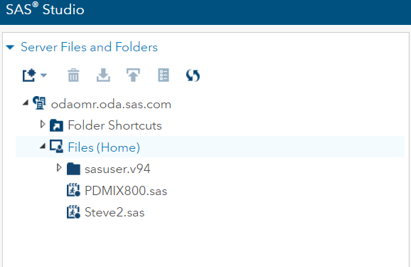
    1. Upload files to SAS Studio.
      • This will place your files within the SAS Studio environment, so that it can see them.
      • To do this – right click on Files(Home)
      • Select Upload Files
      • Select your file and upload

SAS_Studio_Server_Files_Interface.png

2.  Your INFILE statement will need to know where your files are located. They are not on C:\….  they are within the SAS Studio environment.  To find them, right-click on the file and select Properties

SAS_Studio_Server_Files_Properties_Interface.pngSAS_Studio_File_Propertes.png

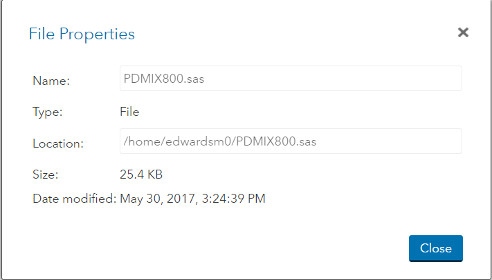
3.  Copy the information in the Location section to use for your INFILE statement.

Data trial;
    Infile “/home/edwardsm0/trial.csv” dlm=”,” firstobs=2;
Input ID$ trmt$ weight height;

Run;

Viewing the data in SAS

We’ve just imported our data and I see nothing!  What happened?  Did I do something wrong?  My log window says my data has been successfully imported, but where did the data go?

Once you’ve imported your data, SAS saved it in a dataset within its program. So think of is as a blackbox and somewhere in that blackbox is a dataset called TRIAL.  How do you go about viewing it?  Let’s use a PROCedure called PRINT.

PROC PRINT will show you your data in the Output window.

Proc print data=trial;
Run;

These statements will printout ALL the observations in your dataset.  Note when we say “printout” it prints to the screen and not to your printer.  Please note that specifying the dataset you are working with is an EXCELLENT habit to get into.  In this case we are interested in viewing the data contained in the TRIAL dataset – data=trial

To view only the first 5 observations in this dataset we can add an option at the end of the Proc print statement.

Proc print data=trial (obs=5);
Run;

Maybe we want to view observations 6-8 we can a second option at the end of our Proc print statements

Proc print data=trial (firstobs=6 obs=8);
Run;

This tells SAS that the first observation we want to view is the 6th observation of a total of 8 observations we are looking at.

We can also tell SAS that rather than looking at all the variables we only want to see TRMT by adding a var statement to our Proc print.

Proc print data=trial (obs=5);
  var TRMT;
Run;

SAS Programming/Coding TIP

1. Add comments to everything you do in SAS.  Use the *  ;  or /*  */  For example:

/*  To test whether I read my data correctly I will use the Proc Print to view the first 10 observations  */

Proc print data=trial (obs=5);
Run;

2.  ALWAYS specify the data that you are using with your PROCedure.

3.  ALWAYS add a RUN; statement at the end of your DATA step and at the end of each PROCedure.  Makes your code cleaner and allows you to select portions of your code to run.

4.  Indenting the lines of code between the PROCedure name and the RUN; statement makes it easier to read your coding.

5.  SAS is NOT case sensitive with respect to your code, however, it is with your data.

6.  The more you code in SAS, the more apt you are to develop your own coding style.

Ridgetown Workshop: Repeated Measures, Adding Year (Location)

For the purposes of this workshop we will work with some fictitious data.  A trial was conducted with 10 reps (blocks), each rep was made up of 5 plots with 1 treatment applied per plot.  Treatments were randomly assigned to the 5 plots within each Rep (block).   Height of each plot was collected on 3 separate days.

Sample Design used in the analysis

The data used in this workshop can be downloaded here.  Please note that the file includes 2 years of data.  We will add the second year of data for our next analysis.

Repeated Measures Analysis

Here is the coding we will use.  I will break apart each line and explain below.

Proc glimmix data=repeated_measures plots=studentpanel;
    by year;
    class rep trmt day PlotID;
    model yield = trmt day trmt*day / ddfm=kr;
     random rep/ subject=plotID;
    random day / subject=plotID type=arh(1) residual;
Run;

Proc glimmix data=repeated_measures plots=studentpanel;

  • Proc glimmix – calling on the GLIMMIX procedure to run our analysis
  • data=repeated_measures – telling SAS which dataset to use – I happened to call mine repeated_measures
  • plots=studentpanel – this requests all residual plots to be displayed after the analysis

    by year;

  • Since we have 2 years of data – rather than breaking up the data into 2 datasets, we will ask SAS to run the analysis separately for each year – by using a BY statement inside the PROC

  class rep trmt day PlotID;

  • listing out our classification variables – or the variables which tell us what group each of our observations fall into

    model yield = trmt day trmt*day / ddfm=kr;

  • Our model statement
  • We have an RCBD design where we have taken repeated measures on our experimental unit – the plot.  So we are interested in the trmt effect, the day effect and the interaction between then two.
  • ddfm=kr – adjustment to the degrees of freedom which adjusts for bias **see  below for more information on this.

     random rep/ subject=plotID;

  • Remember we have an RCBD which means we need to let SAS know that our REPs (or BLOCKs) are a random effect in our model.  Since each of our treatments only appears once in each block – there will be NO trmt*rep interaction
  • This random statement tells SAS that our rep is random – we add a subject= part to the random statement to reaffirm to SAS what our experimental unit is – in this case, PlotID

    random day / subject=plotID type=arh(1) residual;

  • The second random statement in this PROC – is to specify the repeated aspect of our design.
  • Day is the variable which tells us where or when the measures were repeated.
  • Subject tells SAS what the experimental unit was – PlotID in this case
  • We also need to tell SAS what type of relationship there is between the measures taken on the experimental units is – type=arh(1).  Also known as the covariance structure.  In this example I have tried a number of them – which you should always do, and select the one which results in the model with the lowest AICC statistic.  In this example arh(1) – heterogenous autoregressive was the best fit
  • residual – tells SAS that you are partitioning the R-side of the error (experimental error) into a portion due to the repeated measures taken within an experimental unit.

The output for this analysis can be downloaded here.  Start from the bottom of the output file for 1 year to review the residuals.  Please note that there are NO normality statistics produced only the plots.  To run the normality statistics you will still need to save the residuals in a new dataset and rung the PROC UNIVARIATE normal with the residuals.  However, reviewing these plots gives you a great starting point.

Once you are “happy” with the residuals, start reviewing the output from the beginning of the PROC GLIMMIX.  Carefully review the Dimensions table:

Dimensions table from the SAS PROC GLIMMIX output

  • G-side Cov. Parameters = 1 – this refers to the random effect of Rep (Block).  Remember G-side is the random variation between our experimental units.
  • R-side Cov. Parameters = 4 – this refers to the random effects within our experimental units – 3 days + residual error
  • Columns in X – how many levels do we have for our fixed effects in our model?  Trmt = 5, Day = 3, Trmt*day = 15, 1 for the overall mean = 24
  • Columns in Z per Subject – our Rep is our random effect and we have 10 reps
  • Subjects (Blocks in V) = 50 – 10 Reps with 5 plots/rep = 50 experimental units
  • Max Obs per Subject = 3 – each experimental unit (plot) was measured 3 times

You should always be able to track back all these pieces of information to your model.  If you are analyzing a repeated measures it is important to ensure that the last 2 lines of this table is correct.  If they are not, then your model is not reflecting a repeated measures analysis of your trial.

Review the second year of this output to ensure it was run correctly as well.

Doubly Repeated Measures – PROC MIXED

So now let’s add in that second year.  We have a trial which was conducted 2 years in a row.  The previous analysis conducted a repeated measures on the data collected each year as a separate analysis and really as a separate trial.  But, we know there is some relationship between the 2 years, since the same location was used and the same treatments, the same experimental units – so there must be a relationship and we must account for it somehow.

There are 2 ways to handle this at the moment in SAS.  The first way we will look at is treated it as a truly doubly repeated measures – if you think about it – we have the days repeated and we have the years repeated.  Now GLIMMIX cannot necessarily handle this IF there are 2 covariance structures that need to be used – One for Year and one for day, but MIXED can – by using a Kronecker product covariance structure.

Proc mixed data=repeated_measures covtest;
    class rep trmt day PlotID year; 
    model height = trmt day trmt*day Year year*trmt year*day year*trmt*day/       ddfm=kr;
    random rep / subject=plotID;
    repeated year day / subject=plotID type=un@cs;
    lsmeans year*day;
    ods output lsmeans=lsm;
Run;

Proc mixed data=repeated_measures covtest;
    class rep trmt day PlotID year; 

  • These are the same as our PROC GLIMMIX above with the addition of our Year effect in the CLASS statement

model height = trmt day trmt*day Year year*trmt year*day year*trmt*day/       ddfm=kr;

  • Our model has now been expanded to include the effect of the Year.  We are interested in the main effect of Year, the interaction between year and trmt, the interaction between year and day, and the three-way interaction of year, trmt, and day.  If you think these through you will see that we are indeed interested in the if and how the different years have affected the trmt and the day repeated aspect of our trial.
  • Note that we are treating YEAR as a fixed effect.

  random rep / subject=plotID;

  • same as our GLIMMIX statements above

  repeated year day / subject=plotID type=un@cs;

  • MIXED has a specific REPEATED statement whereas GLIMMIX no longer has this.  Note that the structure of this statement is almost identical to the RANDOM statement we used in GLIMMIX with two changes:
    • There is no need to say RESIDUAL with the REPEATED statement in MIXED
    • We are telling MIXED that we have 2 covariance structures with the type= statement
    • un@cs – tells SAS that we want it to use an UNstructure covariance structure for the 2 years, and a CS(compound symmetry) structure for the 3 day measurements.

  lsmeans year*day;
    ods output lsmeans=lsm;

  • These statements are built the same in MIXED and GLIMMIX – I added them here so we can review the lsmeans

To review the complete output provided by this code, please download and view the PDF file.

Doubly Repeated Measures – PROC GLIMMIX

So as I mentioned earlier GLIMMIX cannot handle the true doubly repeated aspect of some of our experiments – what it cannot do is recognize and implement the 2 difference covariance structures for the 2 repeated effects.  However, what we can do is add YEAR as a random effect into a GLIMMIX and our fixed effect results are similar.

Proc glimmix data=repeated_measures plots=studentpanel nobound;
    class year rep trmt day PlotID;
    model height = trmt day trmt*day Year year*trmt year*day year*trmt*day/ ddfm=kr;
    random rep/ subject=plotID group=year;
    random day / subject=plotID type=cs residual;
    lsmestimate year*trmt “2016 Treatments AandB vs C” -1 -1 2 0 0 0 0 0 0 0 ;
    lsmestimate year*trmt “2016 vs 2017 Treatment A” -1 0 0 0 0 1 0 0 0 0 ;
Run;

Proc glimmix data=repeated_measures plots=studentpanel nobound;
    class year rep trmt day PlotID;
    model height = trmt day trmt*day Year year*trmt year*day year*trmt*day/ ddfm=kr;

  • These statements are the same as the previous GLIMMIX and/or MIXED.  Only difference is that I added the nobound option to allow our random effects to have negative variance.  Everything else is the same!

    random rep/ subject=plotID group=year;

  • This statement tells SAS that our REP is random – we have seen this above in both the GLIMMIX and MIXED coding.
  • But this time we have added a GROUP=option.  This allows us to group the random REP effect within each year.  Essentially adding a rep(year) effect to our model.

    random day / subject=plotID type=cs residual;

  • This is our repeated statement for day – which we have seen already.

    lsmestimate year*trmt “2016 Treatments AandB vs C” -1 -1 2 0 0 0 0 0 0 0 ;
    lsmestimate year*trmt “2016 vs 2017 Treatment A” -1 0 0 0 0 1 0 0 0 0 ;

  • Another new statement that you should be aware of.  The LSMESTIMATE allows us to essentially run contrasts amongst our LSMeans – something we were unable to do with MIXED.
  • Something to consider for future analyses and research questions

To review the complete output provided by this code, please download and view the PDF file.

GLIMMIX – Random rep/ group=year VS Random rep(year)

I mentioned above that the statement  random rep/ subject=plotID group=year;  was similar to adding the rep(year) effect as a random effect.  To show you the differences between the output try running the following code:

Proc glimmix data=repeated_measures plots=studentpanel nobound;
    class year rep trmt day PlotID;
    model height = trmt day trmt*day Year year*trmt year*day year*trmt*day/ ddfm=kr;
    random rep(year)/ subject=plotID ;
    random day / subject=plotID type=cs residual;
    lsmestimate year*trmt “2016 Treatments AandB vs C” -1 -1 2 0 0 0 0 0 0 0 ;
    lsmestimate year*trmt “2016 vs 2017 Treatment A” -1 0 0 0 0 1 0 0 0 0 ;
Run;

random rep(year)/ subject=plotID ;

  • This is the only line that is different.  Similar to above – we are adding the random effect of rep(year), and reminding SAS that our experimental unit is plotID but specifying this as the subject

Differences in the output of the 2 previous analyses:

  1. random rep/subject=plotID group= year;  provides 2 G-side covariance parameters – one for each year.  Whereas the random rep(year) / subject=plotID; only provides one parameter the rep(year) effect
  2. AICC for the group=year model = 1638.32, whereas the AICC for the rep(year) model =1656.04.  Suggesting that we are doing a better job with the group=year model.
  3. Since we have different number of covariance parameters, we will have different estimates:cov_GLIMMIX
  4. Overall the Type III Fixed effects for the 2 models were identical

DDFM=KR

We see this added to many of our models and let’s be honest, we ask ourselves WHY?  Is this something I should be adding or not?  When should I be using this?

A quick review

Mixed methods were developed in the 1980-1990s and there has been a lot of research surrounding these methods.  Especially surrounding the are of small sample sizes – now this is a relative term and I will not provide any thoughts as to what is referred to by small sample sizes.

Research has found that when estimated variance and covariance parameters are used to calculate statistics, such as the F-statistic, the results are often biased upward, while the standard error estimates used to calculate confidence intervals are often biased in the opposite direction or downwards.  What does this mean?  We have a higher F-statistic – greater chance of seeing differences, and a small confidence interval.  Now these trends tend to happen when we use mixed methods – which most of us are today.

Research has shown the following trends:

  • There is NO problem when we have balanced designs with a FIXED effects model
  • There is a slight problem with we have unbalanced designs with a FIXED effects model
  • A BIG problem when we have more complex models

So, we can play it safe and use the DDFM adjustment for all of our models.  Let’s be honest, we may have small sample sizes, and we may never be sure whether our model is one that is considered complex or not.

It has been recommended that adding the DDFM=KR should be something that becomes second nature to us and should be added to all of our MODEL statements in GLIMMIX.

Name

ARCHIVE: Summer 2018 Workshops

Workshops for the Summer 2018 have just been posted and are now available for Registration.  Please register if you are planning on attending.  If you register and need to cancel, please do so with the link on the confirmation email you receive when registering or by emailing oacstats@uoguelph.ca .  The registration link for each workshop is listed below and is unique to that workshop.

SAS

A 2-day workshop will be held on May 8-9, 2018 from 9am – 4pm in ANNU Rm 102.  Topics covered will include:

  • Getting the data in
  • Merging datasets and creating new variables
  • Descriptive statistics
  • ANOVA using GLIMMIX – we will work through a number of examples

If you are new to SAS, please plan on attending the 2 days.  For anyone interested in learning more about GLIMMIX, you are invited to attend May 10 only.  However, please note that any material covered on the first day will NOT be repeated on Day 2.

To register for this workshop, please register for each day separately here.

Date: May 8 – 9, 2018 9am – 4pm
Location:  ANNU Rm 102

SPSS

A 2-day workshop will be held on May 16-17, 2018 from 9am – 4pm in ANNU Rm 102.  Topics covered will include:

  • Getting the data in
  • Merging datasets and creating new variables
  • Descriptive statistics
  • ANOVA and GLMM
  • Non-parametric analyses, including Kruskal-Wallis, and Friedman ANOVA

If you want to follow along with the workshop, please ensure that you have the SPSS Software installed on your laptop.  You always have the option to follow the instructor if you do not have the software on your laptop.  Please plan to attend the 2 days to learn all about SPSS and how you can use it for your research project.

To register for this workshop, please register for each day separately here.

Date: May 16-17, 2018  9am-4pm
Location: ANNU Rm 102

R workshop

A 2-day workshop will be held on May 22-23, 2018 from 9am – 4pm in ANNU Rm 102.  Topics covered will include:

  • Getting your data into R
  • Working with your data – cleaning and tidying
  • Descriptive statistics
  • Packages performing ANOVA
  • Packages performing Regression
  • ggplot2

If you want to follow along with the workshop, please ensure that you have the R and RStudio installed on your laptop.  You always have the option to follow the instructor if you do not have the software on your laptop.  Please plan to attend the 2 days to learn all about R and how you can use it for your research project.

To register for this workshop, please register for each day separately here.

Date: May 22-23, 2018  9am-4pm
Location: ANNU Rm 102

RDM: Starting your Research on the Right Foot!

Join Carol Perry from the Library and Michelle Edwards, to learn how to start your research on the right foot.  If you are just starting your graduate work or if you’re an experienced researcher, join us to learn all about the best practices to help you organize and document your project data, store and analyze your data, secure and preserve your data legacy.  This day long workshop is filled with hands-on exercises to encourage you to treat your data as a valuable commodity.  At the end of this workshop, every participant will complete a Data Management Plan and be will be all set to tackle their research data.

This is a one-day workshop held on Tuesday, June 5, 2018 in ANNU Rm 102.  The workshop startst at 9am and will be finished at 4pm.  Please register here.

Date: June 5, 2018  9am-4pm
Location: ANNU Rm 102


Thank-you and hope to see you in a workshop!

Name


Split-split-plot and more experimental designs

Split plot and strip plot (or split block) designs are commonly used in the agronomy, however, they don’t stop there.  We quite often have limited resources and may add on a factor or two on top of our current trial.  This blog post and session will expand on the Split-plot and the Strip-plot (split-block) designs.

Split-split-plot

We have 3 experimental units with 3 differing sizes.  The whole plot, the sub-plot, and the sub-sub-plot.  This link contains a PDF document that displays the Split-split plot design and also contains the Statistical model.

Factor A is the Whole plot – with two levels: A1 and A2.  A1 and A2 are randomly assigned within a block (or rep).  In this illustration we have 2 Blocks (Reps).Main plot of a Split split plot design

The WHOLE plot is now divided into SUB Plots.  Factor B, which has 3 levels is randomly assigned to each level of Factor A in the WHOLE plots.Sub plot of a Split split plot design

The SUB plot is now divided into SUB-SUB Plots.  Factor C, which has 5 levels is randomly assigned to each level of Factor B in the SUB plots.Sub Sub plot of a Split split plot design

Let’s build the model for the Split-Split plot design as modeled above:

Statistical model for a SPlit SPlit plot design

Definition of the Statistical model for the Split split plot design

Split-split-split plot

An extension of the split-split-plot, with a 4th experimental unit.  Same as above 4 differing experimental unit sizes, and therefore 4 errors to be aware of.

Split-plot x Split-block (strip-plot)

The combinations do not seem to end.  The more we look into these designs, the more I realize that many trials that we currently conduct may not be what we think they are.

In this case we are looking at the Split-block or Strip-plot design and within each row/column combination we are adding a third factor within this experimental unit and will aim to randomly assign them – leading us to a Split-plot x split-block design.

I will update with a picture of a design and the statistical model that accompanies it.


Conclusion

After working through these three examples, which design do you think you truly have?

I propose for the last workshop session in April, that we review Latin Square designs, and the combination of Split-plot and latin squares, as I suspect this will talk to a few researchers 🙂

Name

Experimental Designs

What is an experimental design?

Is the process of planning a study to meet specified objectives.  An experiment that SHOULD be designed to match a specific research question.

Steps to designing an experiment

  1. Define the EXPERIMENTAL UNIT
    What is the difference between an EXPERIMENTAL UNIT and a SAMPLING UNIT?
  2. Identify the types of variables
  3. Define the treatment structure
  4. Design the design structure

Experimental Unit  vs. Sampling Unit

Experimental unit is the unit to which the treatment is applied to.

Sampling unit is a fraction of the experimental unit.

Examples of potential experimental units:

  • An animal
  • A cage with 5 birds inside
  • A plot in a field
  • A box of fruit
  • A tree
  • A pot of plants
  • A growth chamber
  • A fish tank
  • A tray of seedlings
  • A taste panelist
  • A sample of a new food product
  • A bench in a greenhouse

Examples of potential sampling units:

  • 1 bird in a cage
  • A quadrant in a plot of a field
  • 5 apples from a box
  • A branch or leaf of a tree
  • 1 plant from a pot of plants
  • A tray or shelf placed in a growth chamber
  • An individual fish from a fish tank
  • One pod of seedlings from a tray
  • A plot on a bench in a greenhouse

Experimental Error

Measure of the variation that exists among observations taken on the experimental units that are treated alike.

Sources of Experimental Error

  1. Natural variation among experimental units
  2. Variability of the measurements taken (response)
  3. Inability to reproduce the treatment conditions exactly from one unit to another
  4. Interaction between the treatments and the experimental units
  5. Any other extraneous factors that may influence the response

With any statistical analyses, what we are looking for is an estimate of the variation of the experimental error.  So, the variation between our experimental units – We need this  to test treatment differences.

Variation of observations within an experimental unit will not give us treatment differences!

Completely Randomized Design (CRD)

Treatments that are randomly assigned to experimental units.

Completely Randomized Design

Experimental unit is the individual plot/square in the design.  The statistical model is represented by:

Model for the CRD

Where:

Yij = Observation on the jth experimental unit on the ith treatment
μ = overall mean
τi = the effect of the ith treatment
εij = experimental error or residual

The experimental error is variation among experimental units on the same treatment. The unexplained variation – the residual – what’s left.

Randomized Complete Block Design (RCBD)

In any experiment we conduct, we have experimental error.  Our goal is to take control over our experimental error so we can study the effects of our treatments.  Blocking is one way to take control of our experimental error.

Blocking occurs when we group experimental units in a way where the variation of the experimental units within the blocks is less than the variation among all the units before blocking.

Diagram of a Randomized Complete Block Design (RCBD)

Each block highlighted as the different colours or the columns in the above table.  Within each block all the treatments will appear an equal amount of time.  The statistical model would be:

RCBD model

What happens though when we have more than one experimental unit/treatment in each block?  If you look at the current design – you have one measurement per treatment in each block – so there is not enough measures to see whether the treatments are doing something different across the blocks.  But when we have more than one experimental unit per treatments in a block, then you have variation to examine.  So your model would now be:

RCBD model with an interaction

Split Plot Design

A design where you have 2-3 factors or treatments of interest, yet the experimental units of each treatment are different sizes.

Split_plot design

What are the 2 sources of experimental error?

Variation between the Blocks where A was assigned.  Two blocks have the A1 treatment and two blocks have the A2 treatment.  The main plot is the A treatment.

The second source of experimental error is the variation among the experimental units.  The subplot is the B treatment.  The statistical model is:

Split_plot model

Split Block or Strip-plot

Two treatments that are applied as a strip as an example.  Here is one blockstrip_plot design

If we are interested in looking at the effect of Treatment A – what is the correct error term?  Start by asking yourself what is the experimental unit for treatment A?  Then think about the definition of experimental error – variation between experimental units that were treated the same….

What about Treatment B?

And the interaction between Treatment A and Treatment B?

The statistical model is:

strip_plot model

Let’s see how much we can get through.

Name